Calculating depreciation is addressed in Chapter 6. For more detailed information, please refer to the chapter.
If so, use age-based depreciation.
If so, use non-linear benefit consumption.
If so, use condition-based depreciation.
Age-based depreciation, also known as straight-line depreciation, assumes a linear increase in depreciation as a function of the asset’s actual age over the asset’s useful life.
- Simple to calculate for new assets
- Requires few additional assumptions
- Historic data may not be available to estimate age, especially for asset components
- Data on last treatment may be necessary to establish age
- Step 1 – Compile Data:
For each asset class and type of component being valued, compile the available data on the asset inventory and its age. Also compile the key parameters established through prior steps, such as useful life and residual value. If treatments other than asset purchase, construction/reconstruction are included, compile the available data on asset treatment history. The assumptions developed previously regarding the level of detail in the analysis and treatments to include may need to be revisited based on what data are available.
- Step 2 – Determine Asset Age:
Specify age at the level of detail established for the calculation – e.g., by individual asset or as a distribution of ages for the inventory. Refer to Chapter 13 of Measuring Capital (11) for guidance on estimating age distributions based on useful life if age data are unavailable.
- Step 3 – Calculate Depreciation:
Use the following equation to calculate depreciation D at time t:
\begin{align*} D(t) &= \frac{(V(t_0)-RV) * (A(t) - A(t_0))}{UL - A(t_0)} \end{align*}
where:
V(t_0) =value at time t_0;RV =residual value;UL =useful life;A(t) =asset age at time t;A(t_0) =asset age at time t_0;Note that when the initial value is based on current replacement cost and residual value is 0 this simplifies to the following:
\begin{align*} D(t) &= \frac{Replacement Cost * A(t)}{UL} \end{align*}
An agency has a bridge, initially constructed in 1960 with an expected lifespan of 70 years. In 2010, the asset was reconstructed and brought back to “like new” condition, resetting the its age to zero in 2010. The replacement cost of the bridge, in today’s dollars, is $5 million with a residual value of $1 million. The depreciation in year 2021 is calculated using the following formula from section 6.2.1:
\begin{align*} D(t) &= \frac{(V(t_0)-RV) * (A(t) - A(t_0))}{UL - A(t_0)} \newline D(t) &= \frac{(5,000,000 - 1,000,000) * (11 - 0)}{(70 - 0)} \newline D(t) &= 628,570 \end{align*}where:
The new value of the asset is $4.37 million.
This example illustrates that how an age-based approach can be utilized in cases where a treatment has the effect of resetting the age. It is more challenging to apply this approach to a case where a rehabilitation is performed that improves the condition of the asset but does not restore it to “like new” condition.
An agency has installed a set of 100 fareboxes on its buses. Each farebox cost approximately $5,000 in current dollars to install. The agency maintains maintenance records on its fareboxes documenting their condition. However, the agency decides to calculate depreciation based on age given fareboxes typically are replaced on a 15-year cycle as a result of technical obsolescence rather than deteriorated condition.
Based on these assumptions the agency determines that a farebox depreciates by $5,000/15 = $333.33 per year until it reaches 15 years. The table below shows a set of example calculations assuming fareboxes of varying age. Based on the table, the initial value of the 100 fareboxes is $500,000. Depreciation totals $265,000, resulting in a current value of $235,000.
Table 6-2. Example Calculation of Asset Value for an Inventory of Fareboxes
| Age (years) | Count | Initial Value ($) | Depreciation ($) | Current Value ($) |
|---|---|---|---|---|
| 0 | 5 | 25,000 | 0 | 25,000 |
| 1 | 6 | 30,000 | 2,000 | 28,000 |
| 2 | 5 | 25,000 | 3,333 | 21,667 |
| 3 | 4 | 20,000 | 4,000 | 16,000 |
| 4 | 3 | 15,000 | 4,000 | 11,000 |
| 5 | 0 | 0 | 0 | 0 |
| 6 | 11 | 55,000 | 22,000 | 33,000 |
| 7 | 10 | 50,000 | 23,333 | 26,667 |
| 8 | 13 | 65,000 | 34,667 | 30,333 |
| 9 | 9 | 45,000 | 27,000 | 18,000 |
| 10 | 5 | 25,000 | 16,667 | 8,333 |
| 11 | 4 | 20,000 | 14,667 | 5,333 |
| 12 | 7 | 35,000 | 28,000 | 7,000 |
| 13 | 4 | 20,000 | 17,333 | 2,667 |
| 14 | 6 | 30,000 | 28,000 | 2,000 |
| >15 | 8 | 40,000 | 40,000 | 0 |
| Total | 100 | 500,000 | 265,000 | 235,000 |
Unit replacement costs are established by asset class/component using expert judgement and/or industry defaults.
Unit replacement costs are established through a one-time analysis of project data and updated in subsequent years based on inflation.
Unit replacement costs are established through a well-documented process that includes: analysis of project data; assessment of how assets should be grouped for analysis (e.g., by system, material and/or surface type); and a defined update cycle (e.g., once every 1 to 2 years).
Asset purchase or construction and reconstruction are included in the asset value calculations. Supplemental analysis is not performed to consider inclusion of other treatments.
An analysis is performed to determine what treatments to include in the analysis, and what treatments are assumed to occur based on the agency’s life cycle strategy. The analysis is conducted separately from establishing asset life cycle strategies.
An analysis is performed to determine what treatments to include in the analysis, and what treatments are assumed to occur based on the agency’s life cycle strategy. The analysis is conducted as part of the development of asset life cycle strategies and/or strategies are updated as appropriate following the analysis.
Asset age is not well established. Costs by asset class are calculated by year and depreciated without associating costs to specific assets.
Asset or component age is known or can be estimated based on inventory and treatment data, supporting calculation of depreciation at an asset class, asset and/or component level.
Asset age or component age is known or can be estimated based on inventory and treatment data. An analysis is performed of the consumption of asset benefits. A custom pattern of benefit consumption is used if supported by the analysis. Depreciation is calculated based on the selected approach by asset class, asset and/or component.
Asset value is calculated for major assets at an aggregate level as required to support financial reporting and TAMP requirements.
Asset value is calculated for major assets. Either the calculations are performed at an asset/component level or supplemental analysis is performed to confirm use of the approach for aggregating asset value calculations.
Asset value is calculated for major assets. Either the calculations are performed at an asset/component level or supplemental analysis is performed to confirm use of the approach for aggregating asset value calculations. Sensitivity analyses are periodically conducted to show the effect of changes in key analysis parameters.
Asset value is reported in agency documents, including financial reports and the agency’s TAMP, but approaches used in different documents may be inconsistent.
Asset value is reported in agency documents, including financial reports and the agency’s TAMP. Discrepancies between different estimates are documented.
Asset value is reported in a consistent manner in different agency documents, including financial reports and the agency’s TAMP. Multiple approaches for reporting value are used as needed to maintain consistency between documents while satisfying reporting requirements.
Condition is used to estimate the asset’s remaining life, and by extension its effective age. The asset’s depreciation increases linearly as a function of its age adjusted for condition.
- Accommodates a range of treatment options
- Does not require historic data
- Supports evaluation of treatment selection and timing for TAM
- Requires the collection of condition data, often at a component level
- Can be challenging to relate condition to effective age, especially for assets in very good or very poor condition
- Step 1 – Map Asset Condition to Effective Age:
For each asset class and type of component being valued, determine how asset condition relates to age. If condition is the best predictor of remaining life, then a simple function or lookup table can be defined to predict effective age for each feasible condition value. Alternatively, one may predict effective age based on condition, actual age and/or other variables. Refer to NCHRP Report 713 (18) for detailed guidance on modeling asset life.
- Step 2 – Compile Data:
For each asset class and type of component being valued, compile the available data on the asset inventory and its condition. If the calculation of effective age requires knowledge of actual age, also compile data on asset age and prior treatments that impact age. Also compile the key parameters established through prior steps, such as useful life and residual value. The assumptions developed previously regarding the level of detail in the analysis and treatments to include may need to be revisited based on what data are available.
- Step 3 – Determine Asset Age:
Specify effective age at the level of detail established for the calculation using the approach established in Step 1.
- Step 4 – Calculate Depreciation:
Use the following equation to calculate depreciation D at time t:
\begin{align*} D(t) &= \frac{(V(t_0)-RV) * (E(t) - E(t_0))}{UL - E(t_0)} \end{align*}
where:
V(t_0) =value at time t_0;RV =residual value;UL =useful life;E(t) =asset age at time t;E(t_0) =asset age at time t_0;Note that when the initial value is based on current replacement cost and residual value is 0 this simplifies to the following:
\begin{align*} D(t) &= \frac{Replacement Cost * E(t)}{UL} \end{align*}
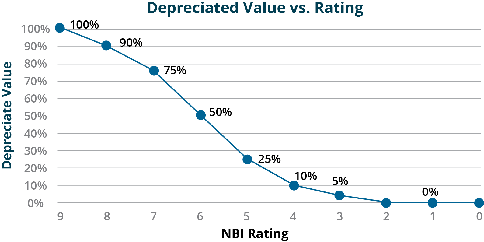
The Kentucky Transportation Cabinet (KYTC) uses a condition-based depreciation approach for valuing assets in its TAMP (37). For bridges KYTC bases depreciation on the NBI condition ratings for the deck, superstructure, and substructure of each bridge. For each value in the NBI scale KYTC has established an equivalent percent of depreciated value, as shown in Figure 6-4.

In Table 6-2 this depreciated value is mapped to an effective remaining service life using KYTC’s assumed useful life of 75 years for a new bridge. The remaining asset life can be substituted into the equation shown in Example 6-1 to calculate depreciation in dollars as a function of condition. The table shows an example of the calculations for a component with an initial value of $10 million.
Table 6-3. Effective Remaining Life and Depreciation Calculations by Condition Rating
| Condition Rating | Depreciated Value (see Figure 6-4) | Effective Remaining Useful Life (years) | Depreciation Given Initial Value of $10M ($M) | Current Value Given Initial Value of $10M ($M) |
|---|---|---|---|---|
| 9 | 100% | 75.00 | 0.0 | 10.0 |
| 8 | 90% | 67.50 | 1.0 | 9.0 |
| 7 | 75% | 56.25 | 2.5 | 7.5 |
| 6 | 50% | 37.50 | 5.0 | 5.0 |
| 5 | 25% | 18.75 | 7.5 | 2.5 |
| 4 | 10% | 7.50 | 9.0 | 1.0 |
| 3 | 5% | 3.75 | 9.5 | 0.5 |
| 2 | 0% | 0.00 | 10.0 | 0.0 |
| 1 | 0% | 0.00 | 10.0 | 0.0 |
Neither historic costs nor asset age can be reliably obtained at an asset level. Overall expenditures by work type and system are used as the basis for calculating asset value without relating expenditures to specific assets.
An asset inventory is available detailing asset age. Historic costs are not reliably tracked by asset but can be estimated using unit replacement costs and asset age
Actual costs of construction/asset purchases are tracked by asset.
The analysis is limited to asset purchase or construction and reconstruction. Asset reconstruction is assumed to have the same cost and effect as initial construction.
Treatment costs are established through a one-time analysis of project data and updated in subsequent years based on inflation. Treatment effects are based on expert judgement or a one-time analysis.
Treatment cost and effects are established through a well-documented process that includes: analysis of treatment data; assessment of how assets should be grouped for analysis (e.g., by system, material, and/or surface type); and a defined update cycle (e.g., once every 1 to 2 years).
Condition data are sufficient for estimating the condition distribution at a network level. Condition is mapped to effective age and depreciation is calculated by asset class based on current condition.
An assessment is performed to determine how best to calculate effective age, potentially using actual age and/or condition. Depreciation is calculated based on effective age by asset class, asset and/or component.
An analysis is performed of the consumption of asset benefits. A custom pattern of benefit consumption is used if supported by the analysis. Otherwise, an assessment is performed to determine how best to calculate effective age, potentially using actual age and/or condition. Depreciation is calculated based on the selected approach by asset class, asset and/or component.
The agency prepares a balance sheet as part of its financial reporting, but does not attempt to reconcile asset value in the financial report with TAM estimates.
Differences in approaches between financial reporting TAM asset valuation are documented as a one-time exercise performed when preparing the TAM asset valuation.
Consistent approaches are used where possible to prepare the balance sheet in the agency’s financial report and value assets for TAM. Differences in approaches are resolved where possible, and regularly reviewed and documented in financial and TAM reports where they remain.
The cost to maintain current asset value is calculated using annual depreciation and reported in the agency’s TAMP.
The cost to maintain current asset value is calculated using the agency’s management systems. The cost to maintain and ASR are reported in the agency’s TAMP.
The cost to maintain current asset value is calculated using the agency’s management systems. The cost to maintain and ASR are reported in the agency’s TAMP. The cost to maintain and ASR are reviewed when establishing asset investment levels.
For non-linear benefit consumption, depreciation is modeled by a set of variables (often age, condition, or a combination of both) representing the consumption of benefits provided by the asset.
- Flexible approach
- Consistent with U.S. and international accounting standards
- Best suited for matching the actual pattern of use
- Requires supplemental analysis
- Results may depend on parameters (e.g. traffic growth) which are outside an asset manager’s control
- Step 1 – Quantify Asset Benefits:
For each asset class and type of component being valued, establish what benefits the asset yields, and how these vary over the life of an asset. Consider agency, user and social costs and benefits, and how these vary over time, as well as based on an asset’s condition.
- Step 2 – Establish the Depreciation Curve:
Determine the functional form of the depreciation curve based on the results of Step 1. If the pattern of benefit consumption can be approximated using a linear relationship, then revert to using a linear model. Otherwise, determine whether the depreciation pattern is accelerated or decelerated relative to linear depreciation.
If the depreciation pattern is accelerated, evaluate whether a fixed depreciation rate can be used, resulting in use of an exponential curve as described in Section 6.1. If the depreciation pattern is decelerated related to linear depreciation, evaluate whether a logistic (s-shaped) curve can be used as described in Section 6.1. Otherwise develop a customized depreciation function.
- Step 3 – Compile Data:
For each asset class and type of component being valued, compile the available data on the asset inventory and other data required to support the depreciation calculation approach defined in Step 2. The assumptions developed previously regarding the level of detail in the analysis and treatments to include may need to be revisited based on what data are available.
- Step 4 – Calculate Depreciation:
Calculate depreciation using the relationship determined in Step 2 with the data compiled in Step 3.
A highway agency is interested in analyzing the pattern of consumption of benefits for pavement. Pavement management staff model the benefit of a pavement section as providing mobility for road users, reducing travel time and operating costs relative to an alternative of using other roads in the event the pavement section was out of service. Over time the use of the pavement increases, in theory yielding greater benefits. However, as the pavement ages roughness increases, reducing benefits obtained from the pavement.
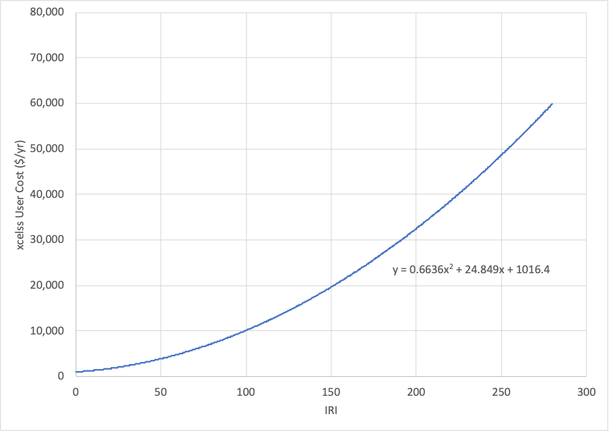
To model these effects the agency staff utilize the model of pavement user costs detailed in NCHRP Report 866 (38). Using the model provided with this report they predict the excess user costs for different representative pavement sections. Figure 6-5 shows the excess user cost as a function of IRI for a 1-mile urban principal arterial with daily traffic of 1,000 vehicles calculated using this model.
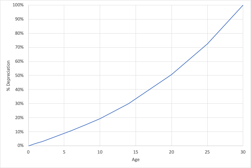
The staff use relationships obtained using the NCHRP report to estimate the benefits realized from a pavement section over time. This is then used to estimate the depreciation curve for pavement. Figure 6-6 shows an example curve for a one-mile section with 1,000 daily vehicles, assuming 5% annual growth in traffic.

